SLAM implementation on a 4 wheeled meccanum robot with a mounted robotic arm
Project documentation
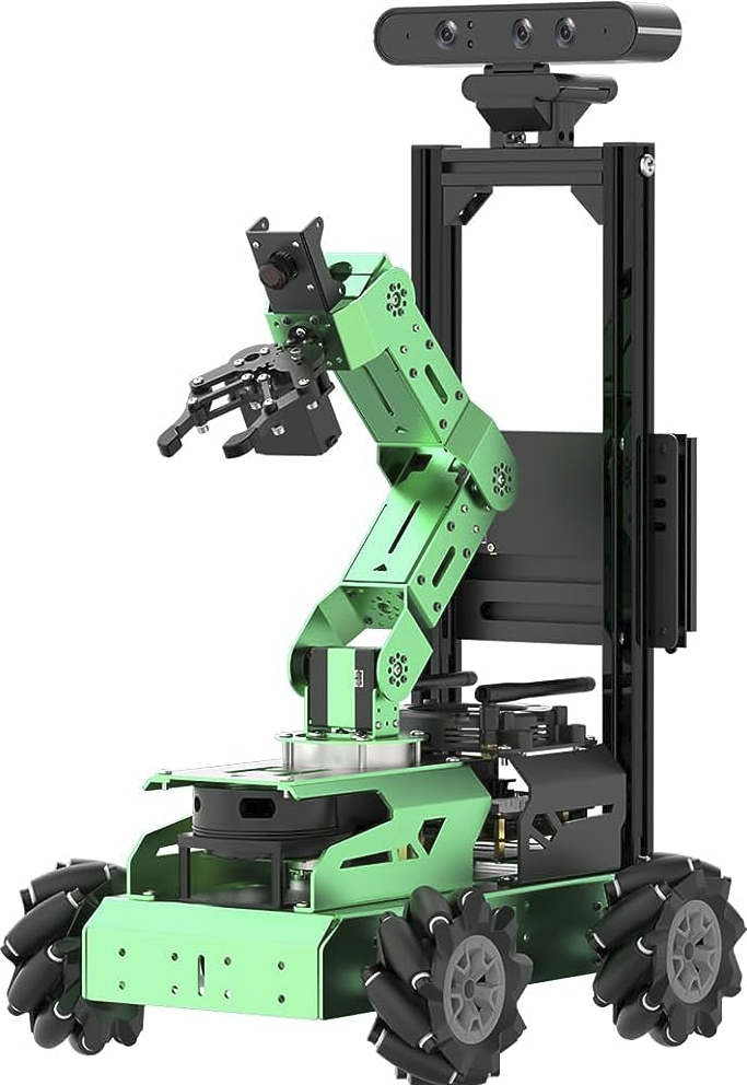
Example of Robot used (Don’t have the original image)
I. Overall Architecture
The robot’s behavior is managed by Robot Operating System (ROS), which uses nodes to control the robot’s actions. The architecture includes a Main Behavior (MB) and Sub-behaviors (SBs). The MB handles high-level logic, communication with SBs, task execution, and error recovery.
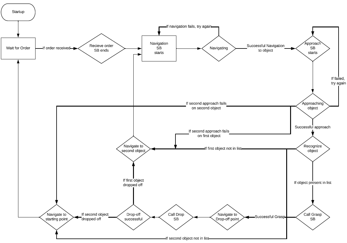
The overall architecture of the domestic service robot
A. States and Transitions
- Initialization: Robot begins in ‘start’ state, loads data, and prepares SBs.
- Receiving Order: MB triggers ‘Receive Order’ SB, awaits input, and gets the list of objects.
- Navigation: Robot moves to home position, then to object locations using ‘Navigate’ SB.
- Approach and Recognize: Robot approaches objects using ‘Approach’ SB, then recognizes them using ‘Recognize’ SB. If unsuccessful, it retries or moves to the next object.
- Grasping: ‘Grasp’ SB calculates object details and guides the arm to grasp it.
- Drop-off: Robot navigates to drop-off point, drops object using ‘Drop’ SB.
- Loop: The process repeats for other objects.
B. Conclusion
At the end of a loop, the robot returns home, publishes dropped object labels, and resets to receive new orders. This completes a full cycle of the behavior.
II. Navigation
To navigate effectively, the robot requires precise knowledge of its position and orientation in the map.
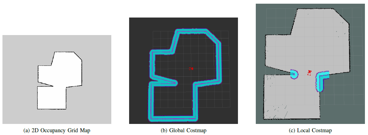
Occupancy Grid and costmaps
A. Sensor Utilization
- The robot employs a Light Detection and Ranging (LiDAR) sensor mounted beneath its base.
- LiDAR measures variable distances by emitting laser pulses and calculating the time taken for reflections to return, creating a real-time map of the environment.
- Simultaneous Localization and Mapping (SLAM) enhances navigation by simultaneously determining the robot’s position and mapping its surroundings.
B. SLAM Implementation
- ROS’s ‘gmapping’ package facilitates SLAM.
- It combines LiDAR data and robot pose information to generate a 2D occupancy grid, which aids in accurate navigation.
C. Map Creation
- The process of creating a 2D grid map involves using MoveBase and ‘map server’ ROS Nodes.
- Gmapping refines the map using LiDAR and odometry data obtained through manual teleoperation.
- Detected obstacles and relative distances from the robot are added to the map during this refinement.
D. CostMaps
- Navigation utilizes two types of costmaps: one for global planning and another for local planning and obstacle avoidance.
- Cost values ranging from 0 to 255 designate objects and empty spaces in the environment.
- The global costmap incorporates information from the initial static map, while the local costmap factors in real-time sensor data.
E. Dijkstra’s Algorithm
- Dijkstra’s algorithm determines the shortest path between nodes in a graph.
- It is applied to the 2D occupancy grid, where each grid box represents a node.
- The algorithm calculates optimal paths by considering weighted edges (distances) and obstacles.
III. Object Recognition
A. Sensors Used
- The robot utilizes an RGB-D Camera, which combines RGB color and depth information on a per-pixel basis.
- Using infrared light, the sensor calculates the time taken for light to bounce back from objects, generating depth data.
- This camera is positioned atop the robot, focusing on the area in front of it to detect objects.
B. Creation of Datasets
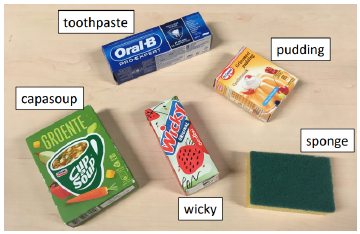
Different objects to be recognized
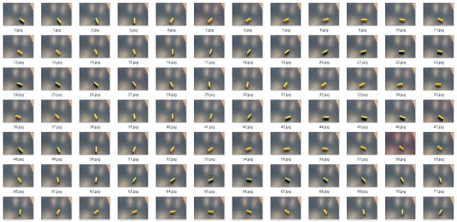
Yaw Rotation for inital dataset
- Initial data collection involves capturing images of five objects using the RGB-D camera.
- Object classes include “cupasoup,” “toothpaste,” “wicky,” “pudding,” and “sponge.”
- Around 120 images of each object are taken from different vertical-yaw orientations.
- A Region-Of-Interest (ROI) program is used to create bounding boxes around objects in images.
- These cropped images are reshaped and used for training a Deep Learning model.
- Data augmentation techniques enhance the dataset for improved recognition accuracy.
C. Deep Learning Model
- Convolutional Neural Network (CNN) operates by applying filters to an input image.
- Convolution and pooling layers reduce image complexity while preserving critical features.
- The CNN architecture employed consists of multiple convolution and pooling cycles.
- Output layer contains nodes corresponding to the five object classes, using a ‘softmax’ activation function for probability assignment.
D. Steps for Object Recognition and Cross-Validation
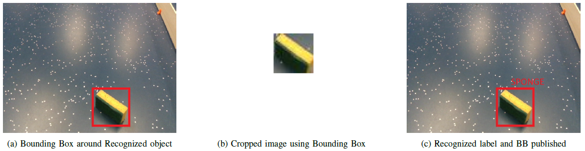
Object recognition and Bounding box
- The robot approaches the object, captures an RGB-D image, and converts it to OpenCV format.
- Using an ROI function, a bounding box is drawn around the object, and the image is cropped and normalized.
The model predicts the object’s class, and if successful, the recognized object’s name is drawn on the image and published to the “/information” topic.
- Cross-validation involves splitting the dataset into K groups to evaluate the model’s performance.
- Over five folds and ten epochs, an average accuracy of 98.14% is achieved on the real dataset.
- The average loss across the ten folds is 5.82%, confirming the effectiveness of the model.
IV. Grasping
The process of grasping objects involves various steps and calculations for precise manipulation.
A. Steps for Obtaining Bounding Box
- A point cloud represents three-dimensional data, including X, Y, Z coordinates and RGB color data.
- Using the RGB-D camera, a point cloud is generated with depth and color information.
- The largest flat surface, typically the floor, is identified and removed from the point cloud.
- The remaining points belong to the object, and PCA is used to calculate its angle with respect to the robot’s base.
- The eigenvector’s angle indicates the object’s yaw.
- The centroid of the object is calculated using the average X, Y, Z values.
- Length, width, and height of the bounding box are determined based on coordinate differences.
- A bounding box is positioned around the object using the calculated dimensions and centroid.
B. Collision Models
- Collision models aid in avoiding obstacles and accurate object positioning.
- Key collision models include the robot’s base, manipulator arm with gripper, object, and the floor.
- They guide the arm’s trajectory and help confirm successful grasping.
C. Steps for Grasping Object
- Grasping begins once an object is successfully recognized and a bounding box is obtained.
- In the MoveIT planning scene, previous collision models are cleared.
- Collision models for the floor and the object to be grasped are added.
- Object’s distance from the robot, dimensions, and angle are sent to the grasp planner.
- MoveIT calculates grasping width and gripper angle for successful manipulation.
- The object is grasped, and the arm returns to the resting position while holding it.
D. Steps for Dropping Object
- Upon reaching the drop-off point, the arm checks for collisions in the environment.
- The arm extends in front of the robot, opening the gripper to drop-off the object.
- Collision models are removed, and the gripper closes as the arm returns to the resting position.
- The robot navigates to the next checkpoint after the drop-off.